
Switching from Sieves to Laser Diffraction
Abstract
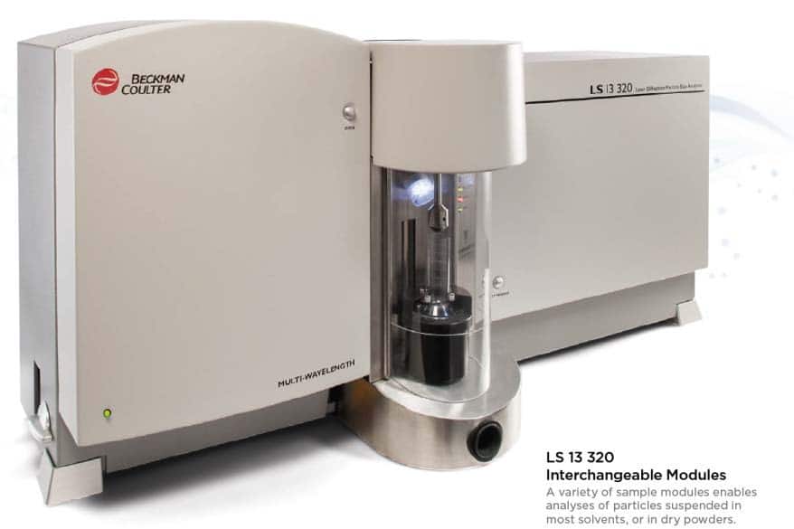
Laser Diffraction offers several advantages over traditional sieve measurements. These include speed, accuracy, low operator to operator variability, ease of use, and quieter operation. Frequently, users understand the advantages of laser diffraction, but are resistant to adopting the technique because they have significant historical data in the sieve format. That is, they are comfortable seeing their results displayed as a weight fraction vs. sieve mesh chart. However, laser diffraction plots are typically percentage volume vs. particle diameter. The LS 13320 from Beckman Coulter features powerful tools to aid these users in the transfer from sieves to the superior laser diffraction technique.
Introduction
Sieving and laser diffraction are two very different approaches to achieve the same goal: understanding the relative amounts of is based on the theory of different particle sizes in a given sample. In sieving, particles in suspension are passed through a stack of progressively finer mesh pans. Subsequently, the stack is disassembled and each pan is weighed to determine the percentage of particles trapped at that mesh size.
In laser diffraction, suspended particles flow through a focused laser beam. As the laser light interacts with the particles, a portion of it is scattered in several different angles. The exact angles of scattering are determined by the size of the particles in suspension. Thus, all laser diffraction instruments capture and quantify the intensity of laser light scattered at various angles. Then, using a series of several algorithms and mathematical operations the size distribution of the particles in suspension is back calculated.
Traditionally it has been challenging to directly compare laser diffraction particle size data with that obtained by sieving; this is because of the fundamental differences in the two techniques. The one exception would be if the sample being analysed were perfectly spherical, both techniques under these circumstances could be expected to give similar answers.
As the sample becomes less spherical and more irregular the results obtained would diverge and any direct comparison becomes more difficult. For example a long needle shaped particle may have a length of 50µm and a width of 10µm. If this sample were to be sieved at 20µm, the needle would in all probability pass through the sieve. This kind of material analysed by laser diffraction would give rise to a distribution which was a composite of all the orientations of the material as it was continually passed through the sample cell.
The Beckman Coulter LS control software has the ability to directly and meaningfully compare LS and sieve data by applying weightings based on the recovered sieve fractions. It needs to be understood of course that each set of weightings must be used specifically with the ‘type’ of material the weightings were obtained from originally. This in practice is simple with the LS software as each ‘weighting’ can be stored as a preference and recalled in a matter of seconds.
Examples: Coarse Dust Sample
The following example represents the general technique and approach that should be adopted when performing this correlation. The sample used in this example is a coarse dust with a wide size distribution.
- First, one must ensure the material is sampled correctly and dispersed within the system appropriately. Additionally, an appropriate correct optical model, based on the materials refractive index, should be chosen.
- Once the data has been obtained, the next step is to establish the correct sieve parameters within the software. This is carried out as follows:
1. From the Preferences menu select the Sieve option. - 2. Select the Mesh Sizes tab as shown in Figure 1.
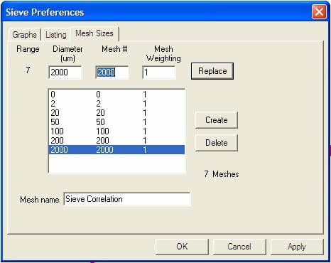
Figure 1 – Sieve Preferences
The values shown represent the ASTM standard sieve set. It will be more than likely they will need to be changed to represent the individual requirements of the user. For instance in this example the following sieve parameters are used:
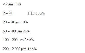
- < 2µm
- 2 µm – 20µm
- 20µm – 50µm
- 50µm – 100µm
- 100 µm – 200 µm
- 200 µm – 2000 µm
To change the sieve sizes, simply highlight each range in turn and type in the appropriate values in the boxes, then press the ‘REPLACE’ button to make the change and the remaining values are then simply deleted.
Some points to note:
- 1. A 0 µm and mesh # of 0 are needed to represents the bottom of the sieve stack.
- 2. Also note that the weighting column currently state 1, this means that the fractions have not yet been weighted.
- 3. You can also fill in the Mesh name option for future reference.
Now we have established the sieve fractions we next need to apply the weighting factors for each fraction. To do this the first step is to load an LS file. The file should represent a ‘standard’ for the material i.e. an example that is acceptable and could be described as ‘normal’. The following steps should be followed:
- 1. Load a file of interest (Figure 2).
- 2. Next select View followed by Sieve.
- 3. Select Graph followed by Cumulative <.
- 4. The final distribution is shown in Figure 3.
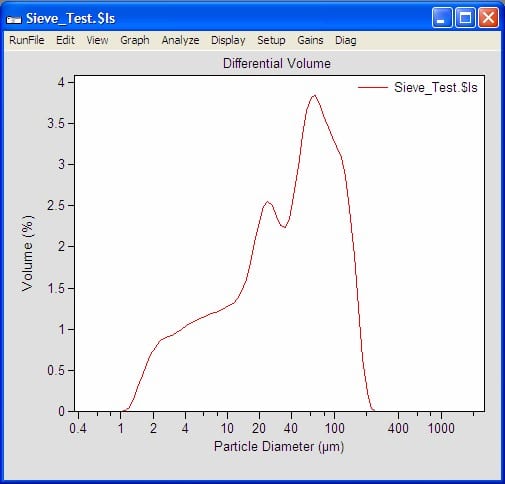
Figure 2 – Representative Size Distribution Data
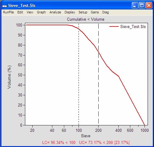
Figure 3 – Data in Figure 2 Plotted as Sieve Data
The next step is to apply the weighting factors for each sieve fraction. Firstly select Edit, and then select Calculate Mesh Weightings. The following dialogue box will be displayed (Figure 4)
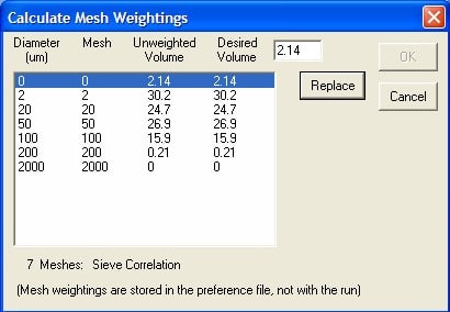
Figure 4 – Mesh weightings dialog screen
Note that the unweighted and desired volume, at first, display the same values. We can now apply the desired weighting factors. The factors are obtained from the sieve data for the sample. In this example, we will use the following values:
To apply the factors simply enter the sieve volumes in the Desired Volume box for each fraction, do this by highlighting each sieve size remembering to press ‘REPLACE’ each time. When completed you should see the following (Figure 5)
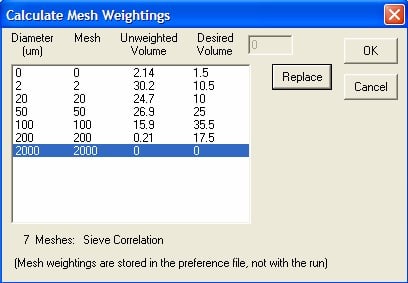
Figure 5 – Mesh weightings volume values
To finish select OK. The distribution will now change to reflect the desired volumes, as shown in Figure 6
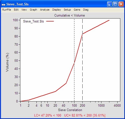
Figure 6 – Sieve correlation graph with correct weighting
It can now be observed that the fraction reported between 100 and 200um is 35.61%. To get a listing of the reported sieve fractions select View and Listings to get all (Figure 7)
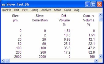
Figure 7– Sieve correlation table output
The last step is to save the weighing as part of the preference file. Simply select Preferences from the main menus, select Save Preferences As; when the save as box appears type in an appropriate name.
Conclusion
This application note explains easy and powerful tool for converting from slow, manual, and cumbersome sieve analysis to fast, reproducible, and easy laser diffraction. The sieve conversion wizard is just one of the many powerful tools contained within the LS 13320 control software.
About the Author
Beckman Coulter Particle Characterization develops, manufactures and markets products that are used to study, analyse and quantify particles of any type. The group serves customers as diverse as cell biologists and cement manufacturers. Serving particle customers since 1960, the group specializes in the Coulter Principle, laser diffraction, dynamic light scattering, zeta potential and automated cell analysis to understand all aspects of particulate samples. For more information, visit www.meritics.com